Setup

The purpose of this analysis is to explore the data, specifically the (i) amount of missingness in potential covariates, (ii) small sample sizes among categories of categorical variables, and (iii) the distribution of potential covariates across the treated and control groups prior to any adjustment. The following R packages are used.

# R packages
library("dplyr")
library("ecdata")
library("ecmeta.nsclc")
library("ggplot2")
library("kableExtra")
library("pins")

# Settings
theme_set(theme_bw())

Data

The underlying dataset used for the analysis is built using the ecdata package. It consists of patients with advanced non-small cell lung cancer (NSCLC) and is documented here. The pins_nsclc() pins the datasets locally using pins::pin() so that the dataset only needs to be built once. We preprocess the data into a format more suitable for propensity score modeling with the preprocess() function and filter to remove the comparator arm from the RCT in order to emulate a single arm trial.

ecdata::pin_nsclc(update = FALSE) # Pins dataset locally
nsclc <- pin_get("nsclc") %>%
  preprocess()
ec_rct1 <- nsclc %>% # Hypothetical single arm trial with external control
  filter(!(source_type == "RCT" & arm_type == "Comparator"))

All pairwise comparisons that will be used in the analyses are displayed in the table below.

analysis <- new_analysis(nsclc)  

analysis %>%
 html_table() %>%
 scroll_box(width = "100%")

		Source		Arm		N
Number	ID	External	Trial	External	Trial	External control	Internal control	Experimental arm
1	nct02008227_fi_1	Flatiron	NCT02008227	Docetaxel	Atezolizumab	526	425	425
2	nct01903993_fi_1	Flatiron	NCT01903993	Docetaxel	Atezolizumab	476	143	144
3	nct02366143_fi_1	Flatiron	NCT02366143	Bevacizumab + Carboplatin	Atezolizumab + Bevacizumab + Carboplatin	602	336	356
4	nct01351415_fi_1	Flatiron	NCT01351415	SOC	Bevacizumab + SOC	381	240	245
5	nct01519804_fi_1	Flatiron	NCT01519804	Placebo + Platinum + Paclitaxel	MetMAb + Platinum + Paclitaxel	1945	54	55
6	nct01496742_fi_1	Flatiron	NCT01496742	Placebo + Bevacizumab + Platinum	MetMAb + Bevacizumab + Platinum + Paclitaxel	956	70	69
7	nct01496742_fi_2	Flatiron	NCT01496742	Placebo + Platinum + Pemetrexed	MetMAb + Platinum + Pemetrexed	3244	61	59
8	nct01366131_fi_1	Flatiron	NCT01366131	Placebo + Bevacizumab + Carboplatin + Paclitaxel	MEGF0444A + Bevacizumab + Carboplatin + Paclitaxel	963	52	52
9	nct01493843_fi_1	Flatiron	NCT01493843	Placebo (340 mg) + Carboplatin + Paclitaxel	Pictilisib (340 mg) + Carboplatin + Paclitaxel	1274	125	126
10	nct01493843_fi_2	Flatiron	NCT01493843	Placebo (340 mg) + Carboplatin + Paclitaxel + Bevacizumab	Pictilisib (340 mg) + Carboplatin + Paclitaxel + Bevacizumab	953	79	79
11	nct01493843_fi_3	Flatiron	NCT01493843	Placebo (260 mg) + Carboplatin + Paclitaxel + Bevacizumab	Pictilisib (260 mg) + Carboplatin + Paclitaxel + Bevacizumab	953	30	62
12	nct02367781_fi_1	Flatiron	NCT02367781	Nab-Paclitaxel + Carboplatin	Atezolizumab + Nab-Paclitaxel + Carboplatin	87	228	451
13	nct02367794_fi_1	Flatiron	NCT02367794	Nab-Paclitaxel + Carboplatin	Atezolizumab + Nab-Paclitaxel + Carboplatin	497	340	343
14	nct02657434_fi_1	Flatiron	NCT02657434	Carboplatin or Cisplatin + Pemetrexed	Atezolizumab + Carboplatin or Cisplatin + Pemetrexed	1536	286	292

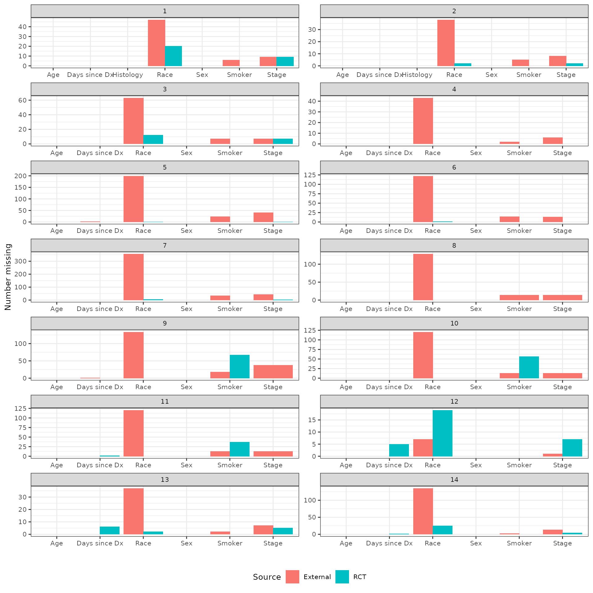
Missing data

We count the number of missing values of each potential covariate for each pairwise analysis. Both the number of missing and the proportion missing (of the total number of observations with each arm) are plotted.

n_missing_df <- count_missing(ec_rct1, vars = get_ps_vars())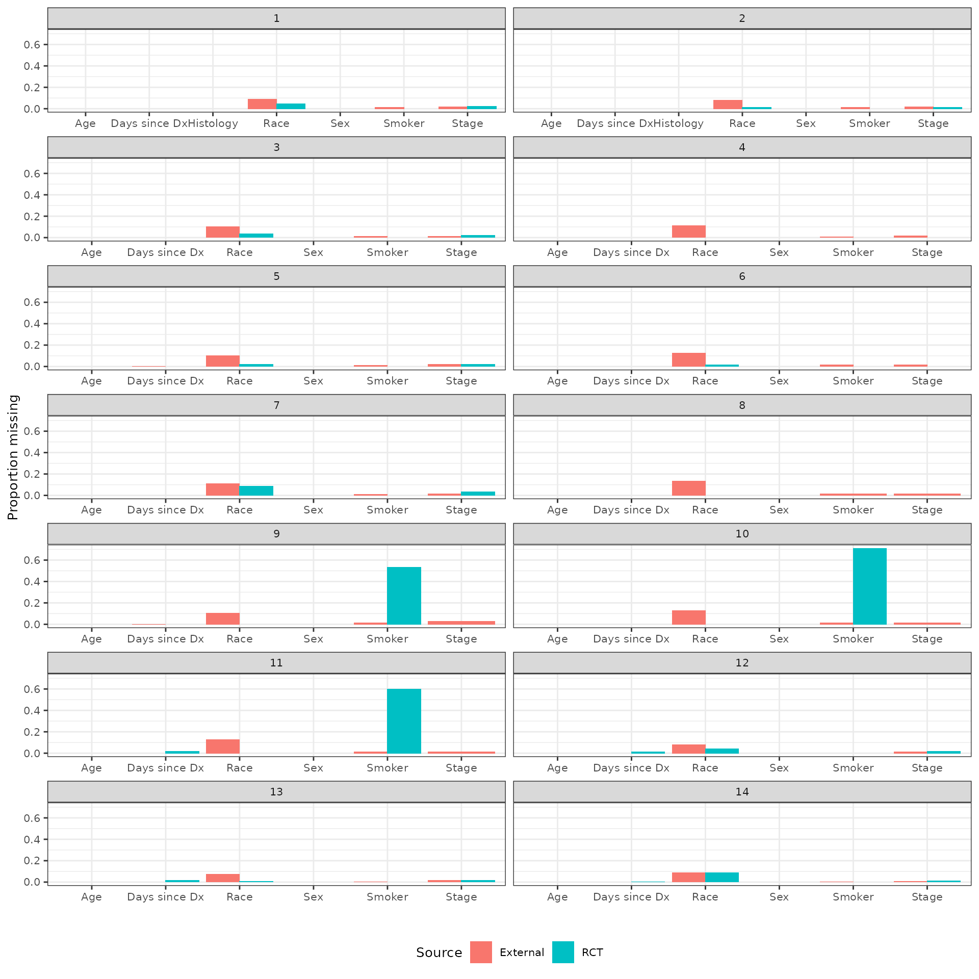

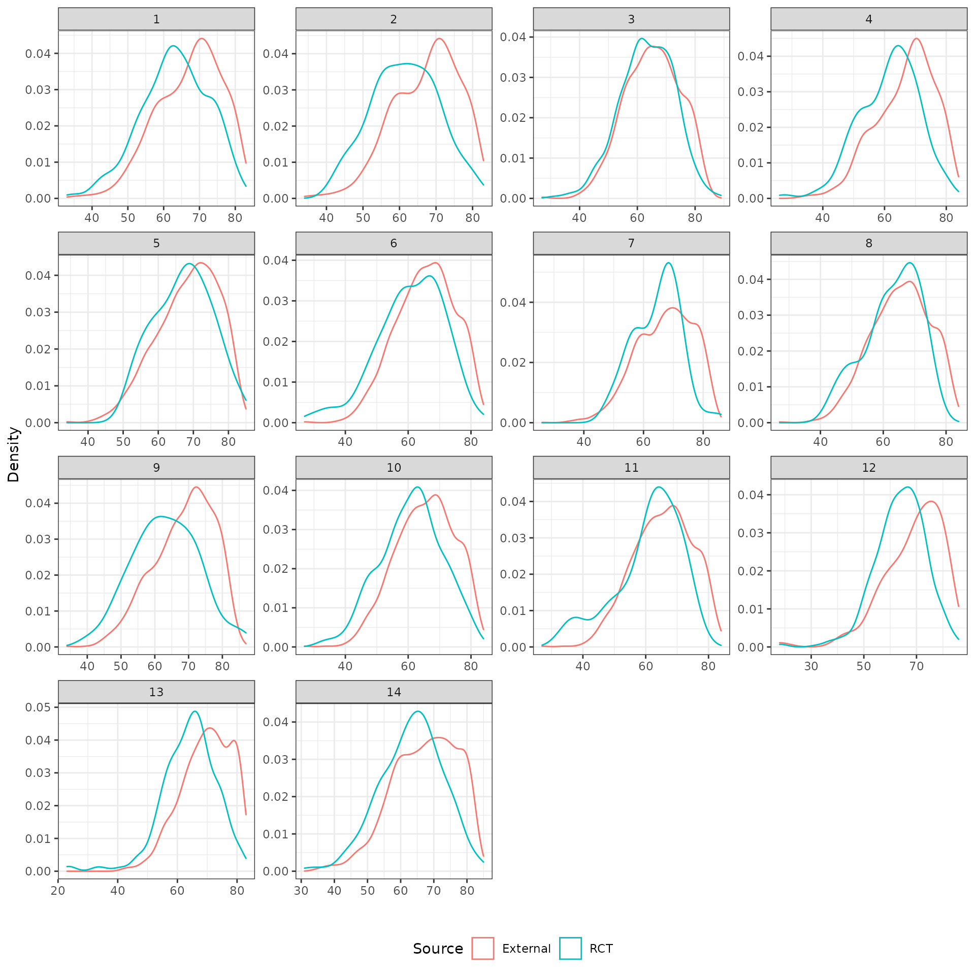
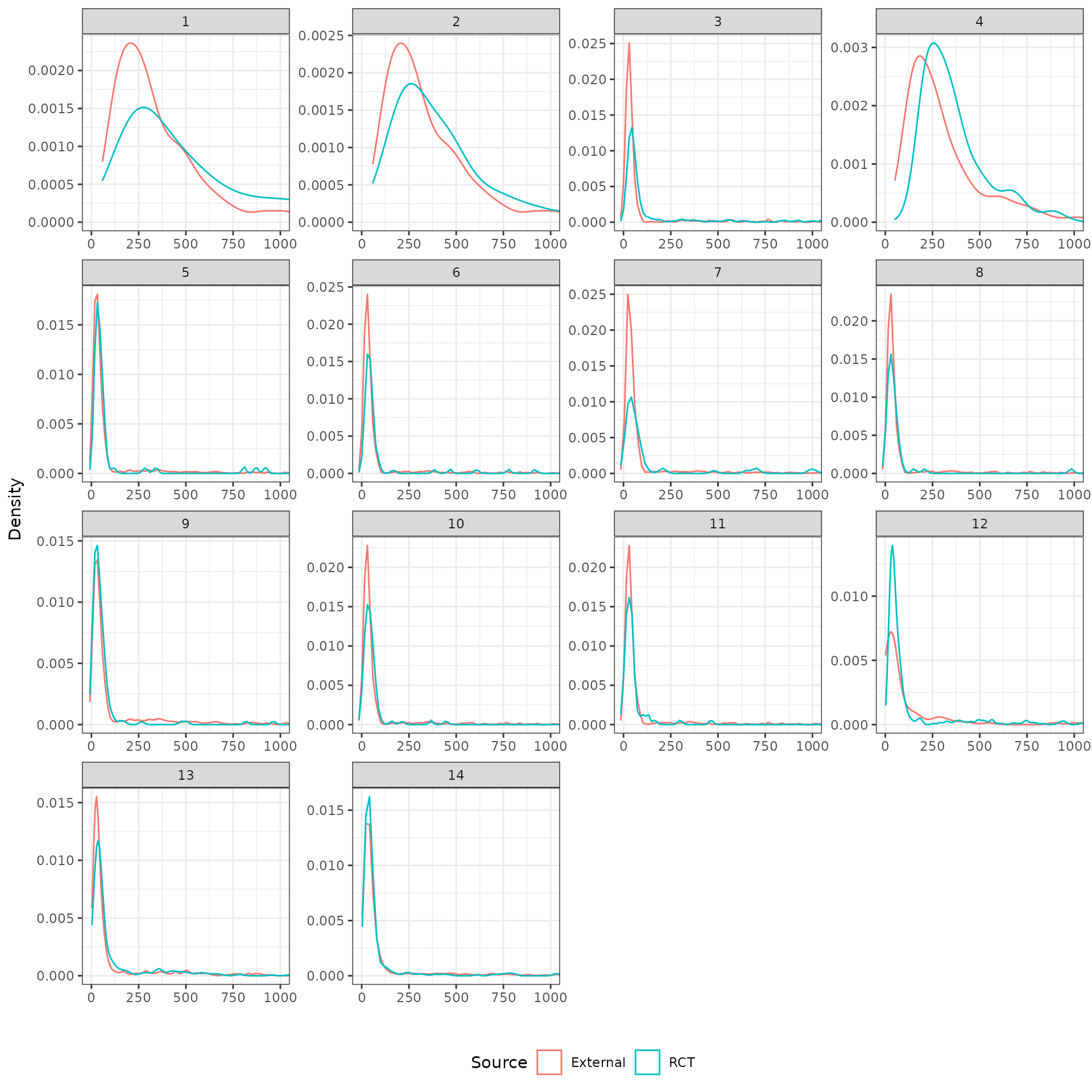
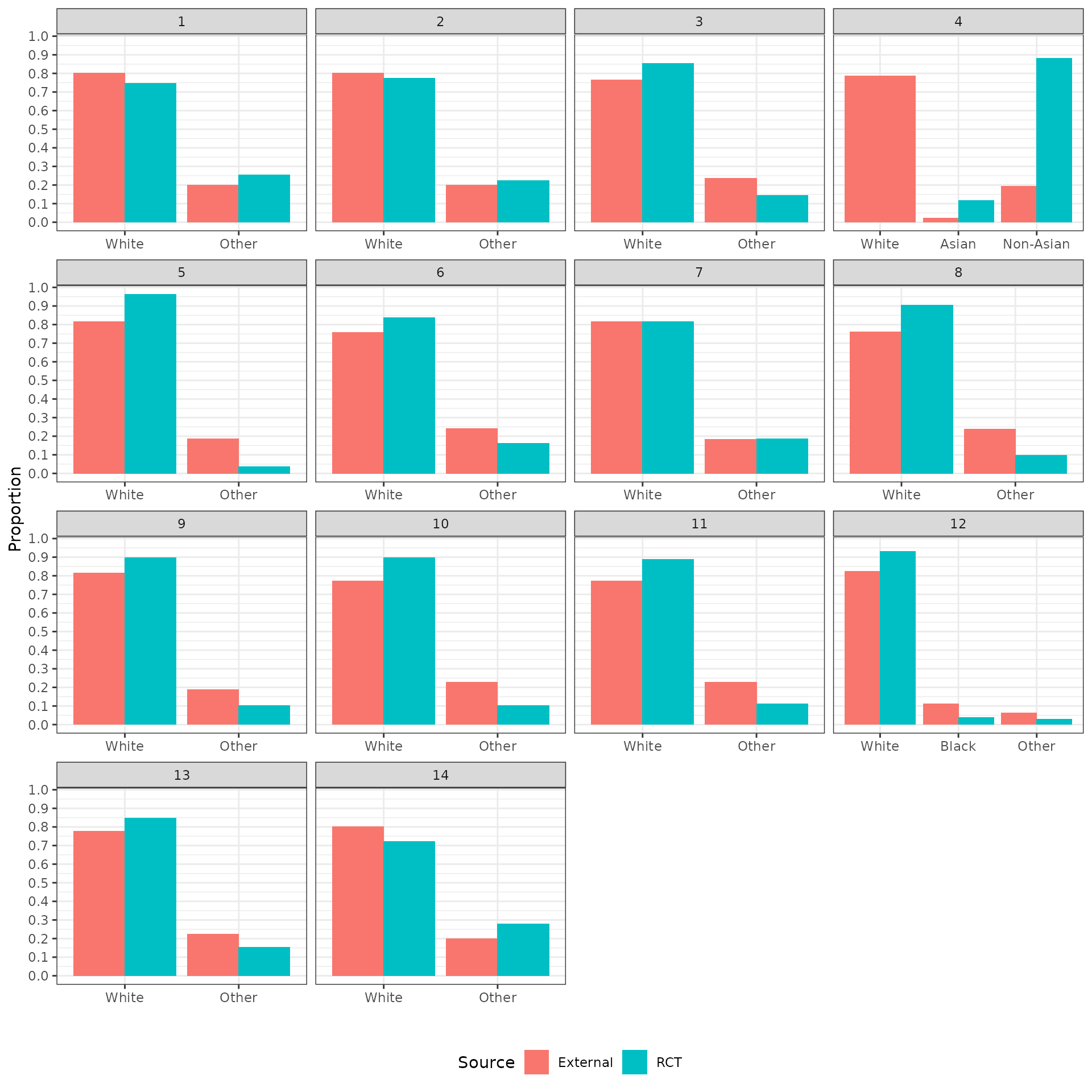
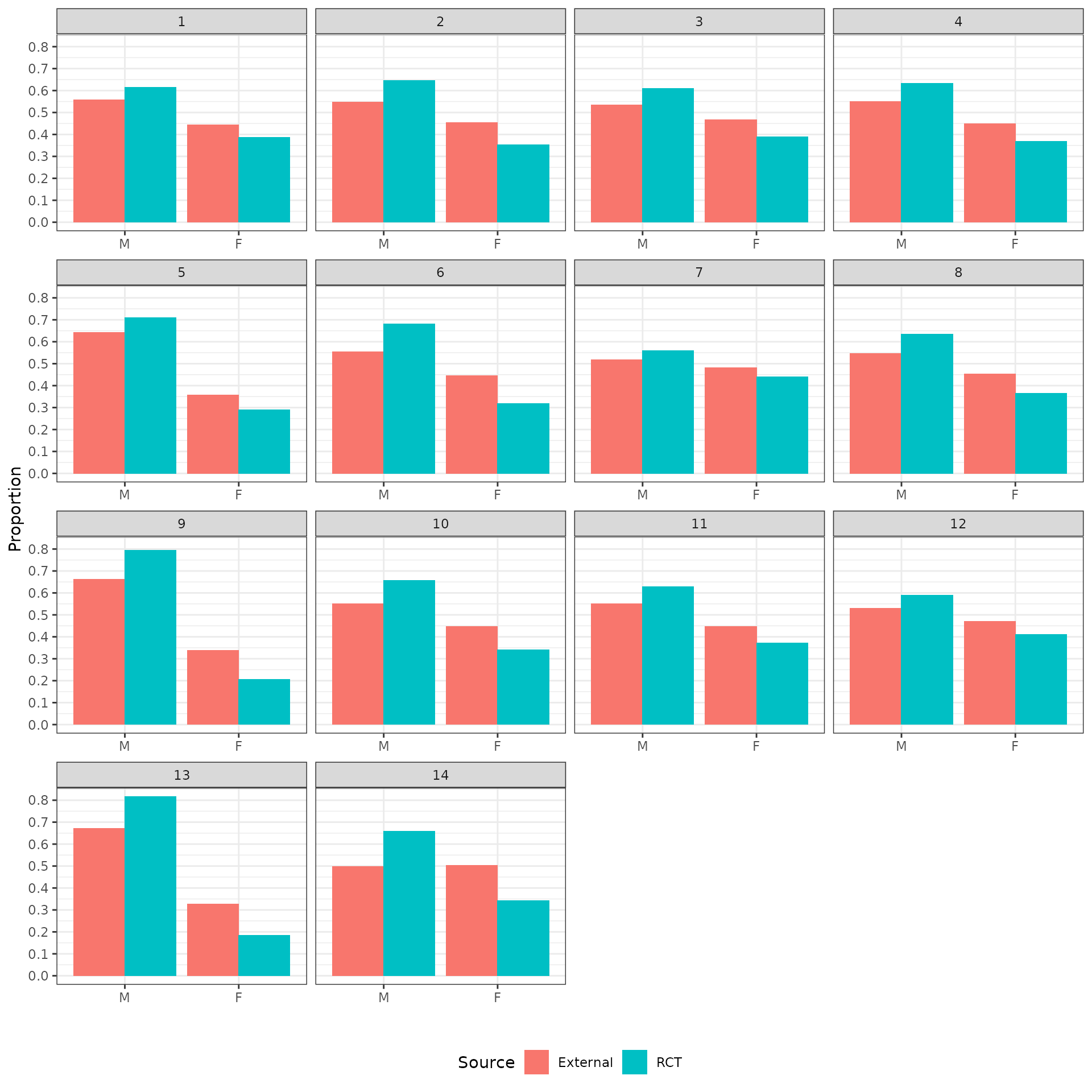
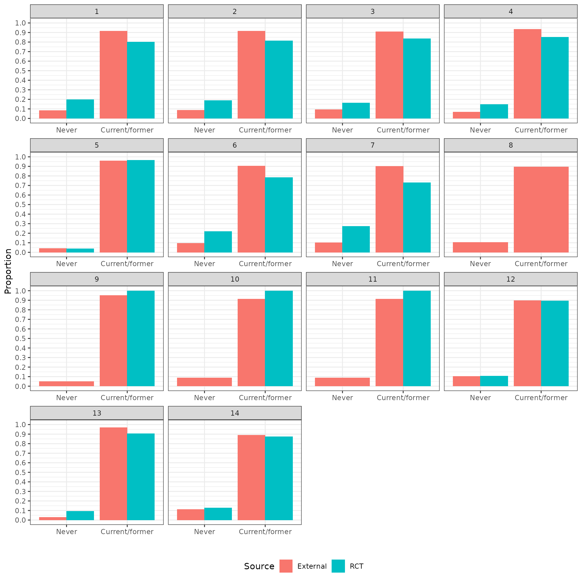
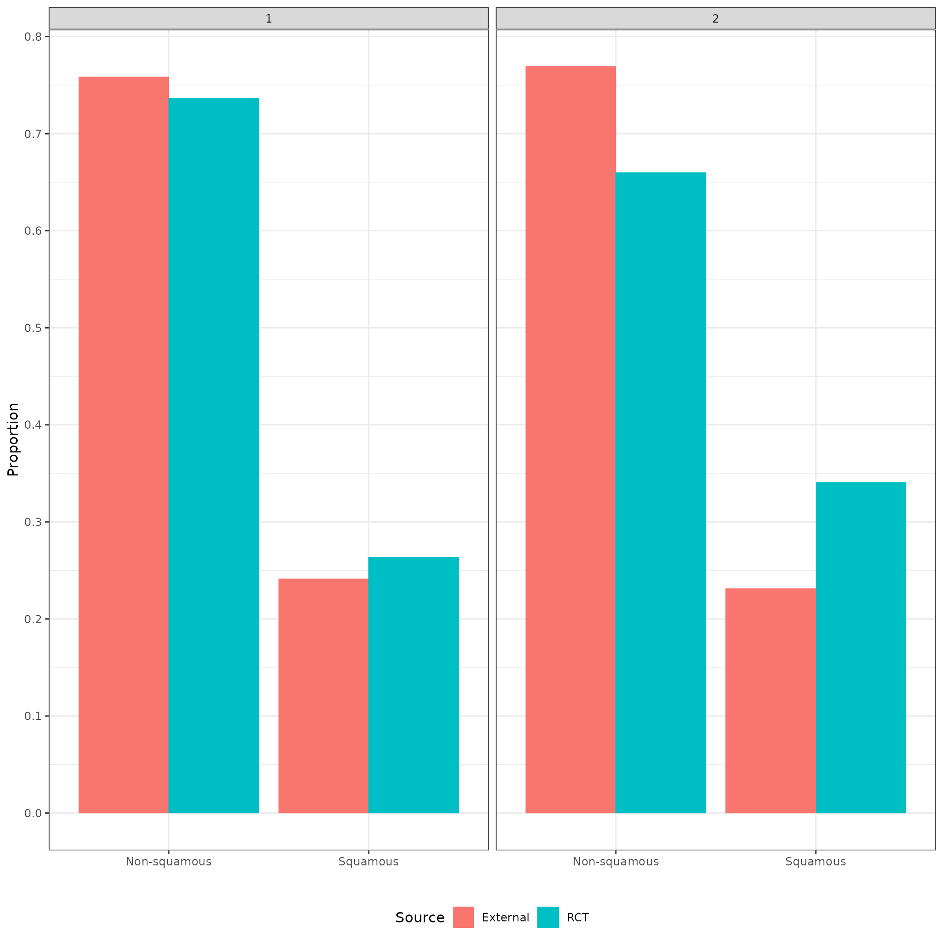
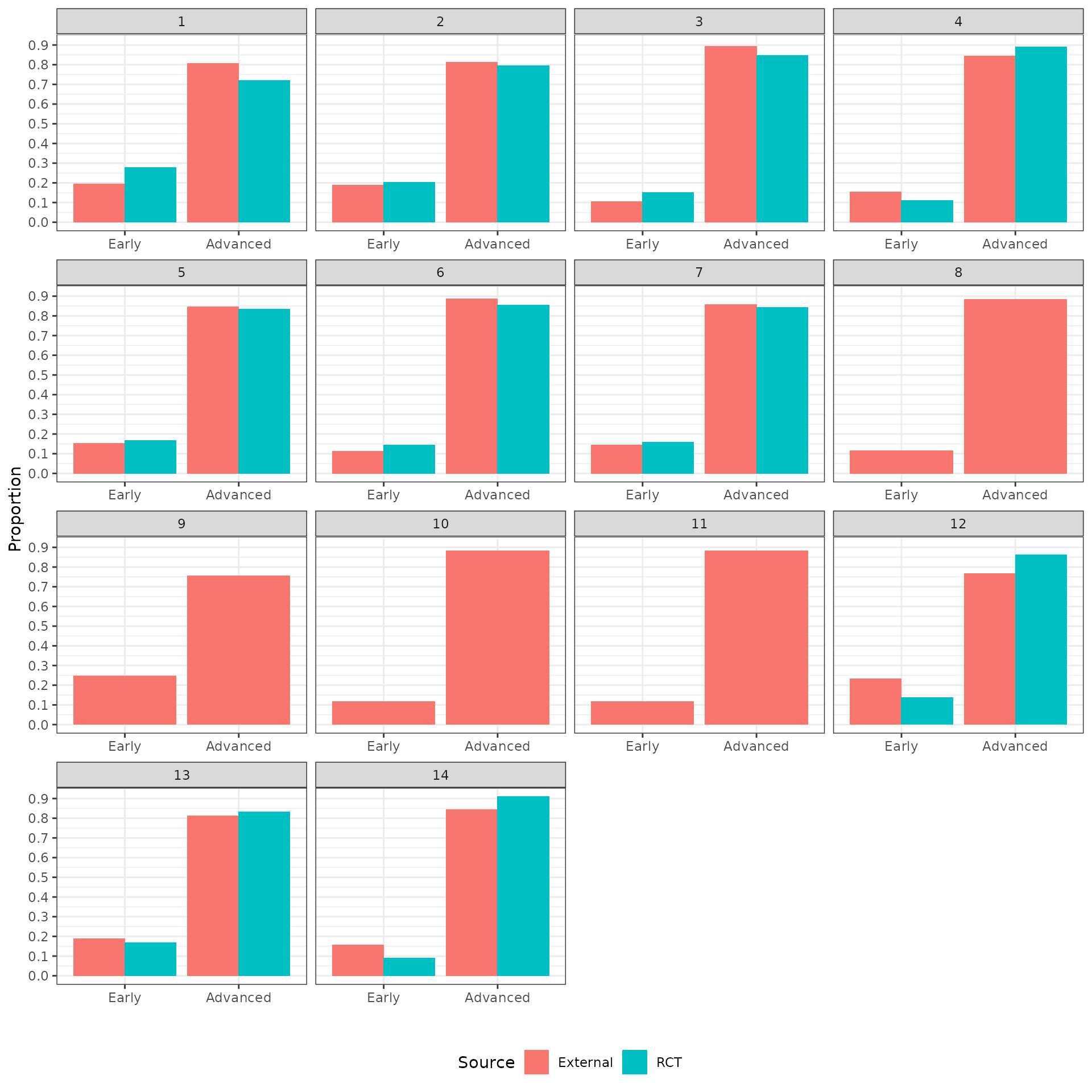
Proportion missing

autoplot(n_missing_df, yvar = "prop_missing")

Number missing

autoplot(n_missing_df, yvar = "n_missing")

Distribution of covariates

The distributions of the covariates in the unadjusted sample are plotted to check the degree of imbalance prior to adjustment and check for outliers or coding errors. There are a couple of points worth noting:

NCT01366131 did not collect smoking information.
It is not possible to determine whether a patient is a “Never” smoker in NCT01493843 because there is only a “Former/never” category. Smoking status can therefore not be used for propensity score analyses for this trial.
Patients in a race category with fewer than 10 observations were coded as “Other” race.

Age

plot_density(ec_rct1, var = "age")

Days since Dx

plot_density(ec_rct1, var = "days_since_dx", xlim = c(0, 1000))

Race

plot_bar(ec_rct1, var = "race_grouped")

Sex

plot_bar(ec_rct1, var = "sex")

Smoker

plot_bar(ec_rct1, var = "smoker_grouped")

Histology

plot_bar(ec_rct1, var = "histology")

Cancer stage

plot_bar(ec_rct1, var = "stage_grouped")

Categorical variables with small sample sizes

The plots above suggest that some categories of the categorical variables might still have small sample sizes even after preprocessing. Categories of categorical variables with fewer than 10 observations are shown in the table below.

count_by(ec_rct1, vars = get_ps_catvars(), 
         by = c("analysis_num", "source_type"),
         max_n = 9) %>%
  html_table()

analysis_num	source_type	var	value	n
4	External	race_grouped	Asian	7
5	RCT	race_grouped	Other	2
5	RCT	smoker_grouped	Never	2
5	RCT	stage_grouped	Early	9
7	RCT	stage_grouped	Early	9
8	RCT	race_grouped	Other	5
10	RCT	race_grouped	Other	8
11	RCT	race_grouped	Other	7
12	External	race_grouped	Black	9
12	External	race_grouped	Other	5
12	External	smoker_grouped	Never	9

Save output

saveRDS(analysis, file = "analysis-data-prep.rds")

Session information

sessionInfo()

## R version 4.0.0 (2020-04-24)
## Platform: x86_64-pc-linux-gnu (64-bit)
## Running under: Ubuntu 18.04.5 LTS
## 
## Matrix products: default
## BLAS:   /usr/lib/x86_64-linux-gnu/openblas/libblas.so.3
## LAPACK: /usr/lib/x86_64-linux-gnu/libopenblasp-r0.2.20.so
## 
## locale:
##  [1] LC_CTYPE=en_US.UTF-8       LC_NUMERIC=C              
##  [3] LC_TIME=en_US.UTF-8        LC_COLLATE=en_US.UTF-8    
##  [5] LC_MONETARY=en_US.UTF-8    LC_MESSAGES=en_US.UTF-8   
##  [7] LC_PAPER=en_US.UTF-8       LC_NAME=C                 
##  [9] LC_ADDRESS=C               LC_TELEPHONE=C            
## [11] LC_MEASUREMENT=en_US.UTF-8 LC_IDENTIFICATION=C       
## 
## attached base packages:
## [1] stats     graphics  grDevices utils     datasets  methods   base     
## 
## other attached packages:
## [1] pins_0.4.5         kableExtra_1.3.4   ggplot2_3.3.5      ecmeta.nsclc_0.1.0
## [5] ecdata_0.2.1       dplyr_1.0.7       
## 
## loaded via a namespace (and not attached):
##  [1] svglite_2.0.0     lattice_0.20-45   tidyr_1.1.4       assertthat_0.2.1 
##  [5] rprojroot_2.0.2   digest_0.6.28     utf8_1.2.2        R6_2.5.1         
##  [9] backports_1.2.1   evaluate_0.14     highr_0.9         httr_1.4.2       
## [13] pillar_1.6.3      rlang_0.4.11      rstudioapi_0.13   data.table_1.14.2
## [17] jquerylib_0.1.4   Matrix_1.3-4      rmarkdown_2.11    pkgdown_1.6.1    
## [21] labeling_0.4.2    textshaping_0.3.5 desc_1.4.0        splines_4.0.0    
## [25] webshot_0.5.2     stringr_1.4.0     munsell_0.5.0     compiler_4.0.0   
## [29] xfun_0.26         pkgconfig_2.0.3   systemfonts_1.0.2 htmltools_0.5.2  
## [33] tidyselect_1.1.1  tibble_3.1.5      fansi_0.5.0       viridisLite_0.4.0
## [37] crayon_1.4.1      withr_2.4.2       rappdirs_0.3.3    grid_4.0.0       
## [41] xtable_1.8-4      jsonlite_1.7.2    gtable_0.3.0      lifecycle_1.0.1  
## [45] DBI_1.1.1         magrittr_2.0.1    scales_1.1.1      stringi_1.7.4    
## [49] cachem_1.0.6      farver_2.1.0      fs_1.5.0          xml2_1.3.2       
## [53] bslib_0.3.0       ellipsis_0.3.2    filelock_1.0.2    ragg_1.1.3       
## [57] generics_0.1.0    vctrs_0.3.8       tools_4.0.0       glue_1.4.2       
## [61] purrr_0.3.4       fastmap_1.1.0     survival_3.2-13   yaml_2.2.1       
## [65] colorspace_2.0-2  rvest_1.0.1       memoise_2.0.0     knitr_1.36       
## [69] sass_0.4.0

Preparation and exploration of external control datasets

2021-10-01