RCT benchmarks
We first obtain RCT datasets for each of the analyses so that we can generate hazard ratio benchmarks for our external control analyses.
Hazard ratios are estimated with Cox models that include a single covariate for treatment assignment. We first estimate log hazard ratios (which we will need for our meta-analytic model) and then transform them to hazard ratios for presentation.
# Estimate log hazard ratios
rct_loghr <- map(rct_list, function(x) {
  fit <- coxph(SURV_FORMULA, data = x)
  loghr <- c(coef(fit), sqrt(vcov(fit)), confint(fit))
  tibble(estimate = loghr[1],
         se = loghr[2],
         lower = loghr[3],
         upper = loghr[4])
}) %>%
  bind_rows(.id = "analysis_num") %>%
  mutate(analysis_num = as.integer(analysis_num))

# Transform to hazard ratios
rct_hr <- rct_loghr %>%
  mutate(across(c(estimate, lower, upper), .fns = exp))
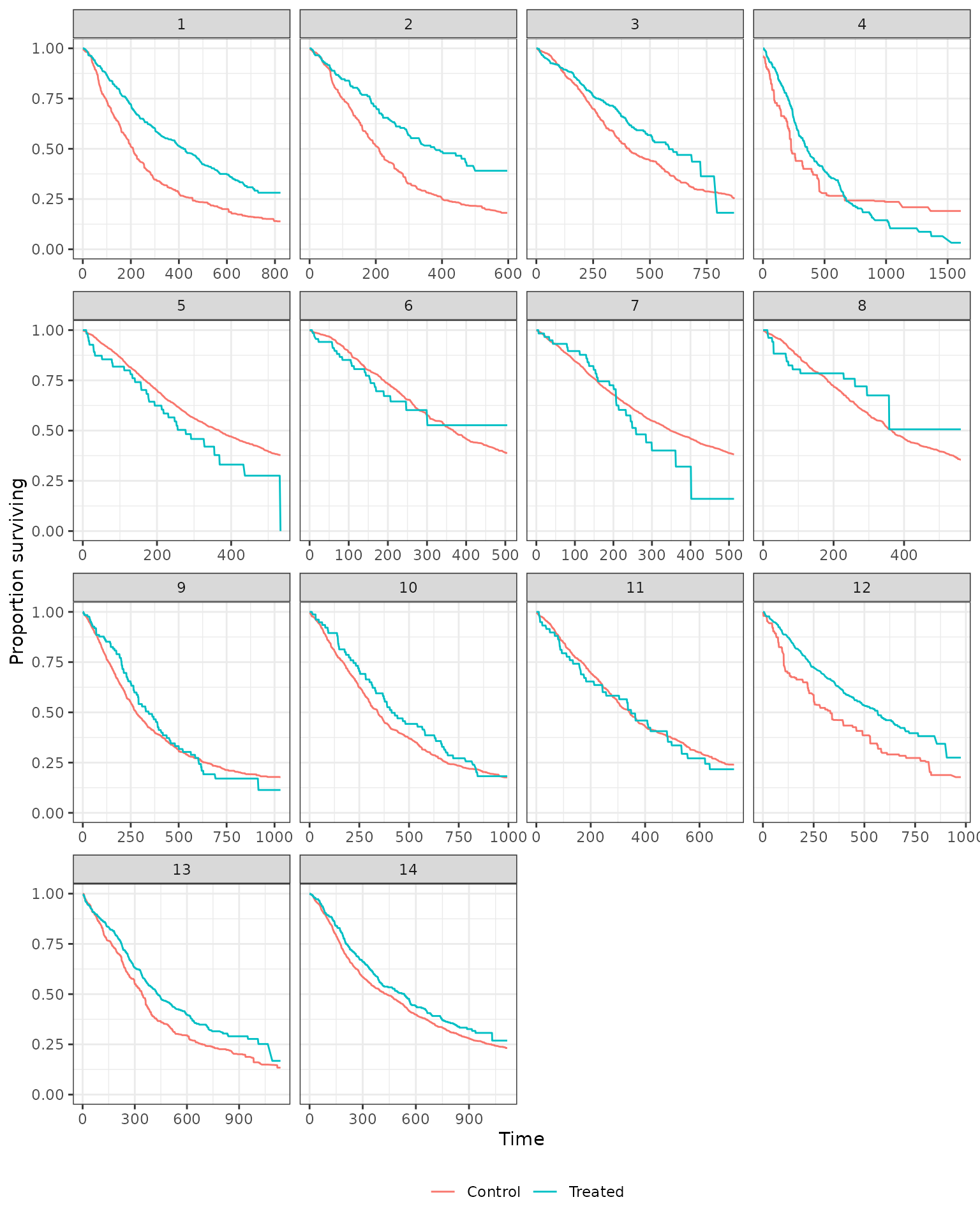
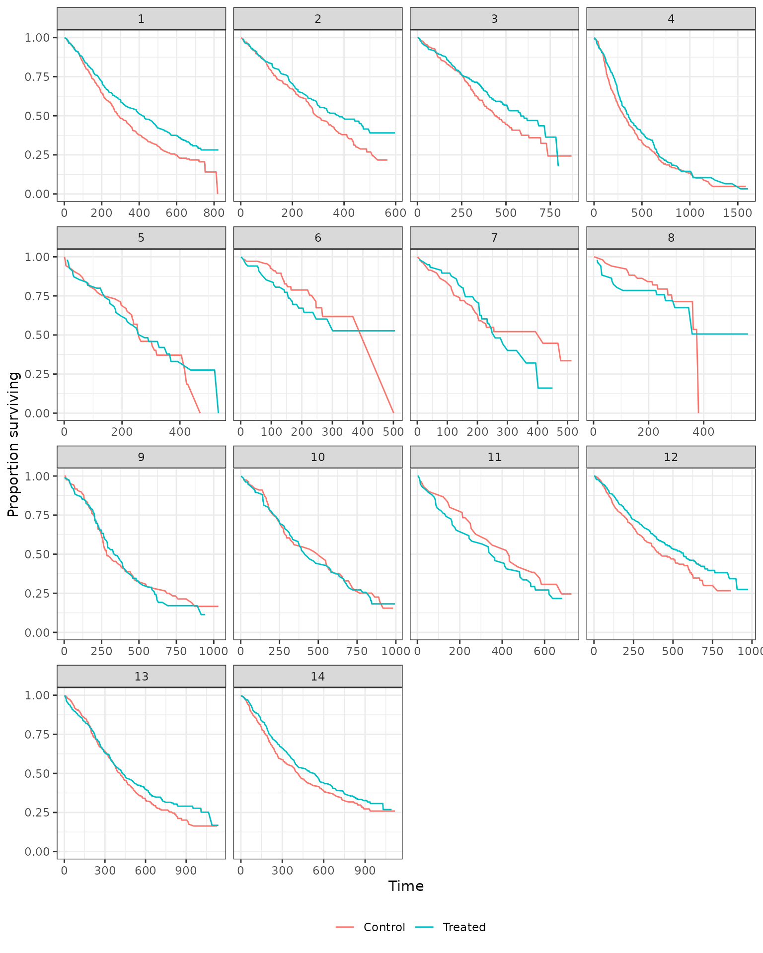
We also generate Kaplan-Meier estimates stratified by treatment assignment.
Sensitivity analyses
A number of sensitivity analyses are performed to assess sensitivity of the results to modeling assumptions.
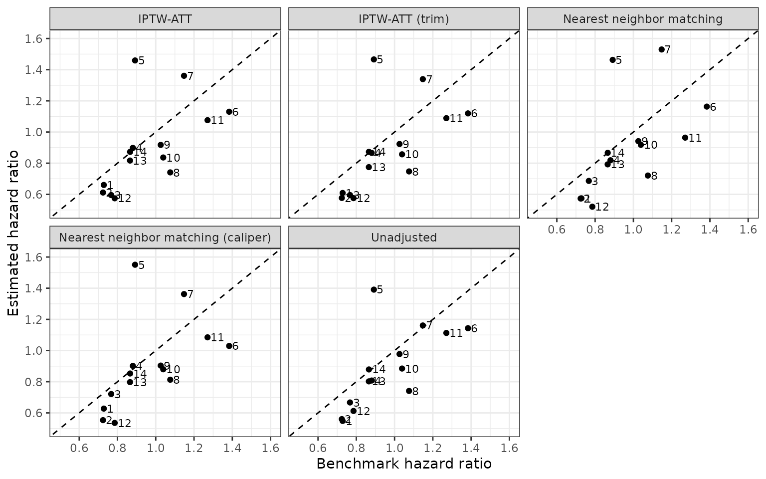
Propensity score methods
The first sensitivty analysis assess the importance of difference propensity score methods.
psmethods_ate <- map_surv_ate(analysis$psweight, ydata_list = y_list,
                              response = RESPONSE, id = ID,
                              grp_id = GRP_ID,
                              integer_grp_id = TRUE)
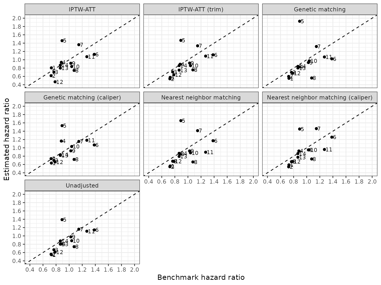
We compare the estimated and benchmark hazard ratios across the difference methodologies.
|
analysis_num
|
term
|
benchmark
|
iptw_att
|
iptw_att_trim
|
match_genetic
|
match_genetic_caliper
|
match_nearest
|
match_nearest_caliper
|
unadjusted
|
|
1
|
treat
|
0.73 (0.62-0.86)
|
0.81 (0.46-1.41)
|
0.58 (0.48-0.69)
|
0.55 (0.47-0.65)
|
0.63 (0.50-0.80)
|
0.56 (0.48-0.66)
|
0.59 (0.49-0.71)
|
0.55 (0.47-0.64)
|
|
2
|
treat
|
0.72 (0.54-0.98)
|
0.62 (0.43-0.88)
|
0.54 (0.41-0.71)
|
0.60 (0.43-0.85)
|
0.74 (0.50-1.09)
|
0.55 (0.40-0.75)
|
0.54 (0.39-0.76)
|
0.56 (0.44-0.72)
|
|
3
|
treat
|
0.77 (0.61-0.96)
|
0.71 (0.58-0.86)
|
0.71 (0.58-0.87)
|
0.70 (0.56-0.87)
|
0.70 (0.55-0.89)
|
0.68 (0.54-0.85)
|
0.67 (0.53-0.84)
|
0.67 (0.55-0.81)
|
|
4
|
treat
|
0.88 (0.72-1.07)
|
0.94 (0.59-1.49)
|
0.89 (0.59-1.34)
|
0.83 (0.68-1.02)
|
1.16 (0.74-1.84)
|
0.85 (0.69-1.05)
|
0.92 (0.62-1.38)
|
0.81 (0.68-0.96)
|
|
5
|
treat
|
0.89 (0.55-1.46)
|
1.46 (1.04-2.04)
|
1.47 (1.05-2.05)
|
1.93 (1.08-3.43)
|
1.53 (0.85-2.76)
|
1.65 (0.94-2.92)
|
1.45 (0.83-2.53)
|
1.39 (0.99-1.95)
|
|
6
|
treat
|
1.38 (0.75-2.56)
|
1.13 (0.73-1.75)
|
1.12 (0.72-1.74)
|
1.02 (0.58-1.80)
|
1.07 (0.62-1.85)
|
1.17 (0.64-2.13)
|
1.26 (0.67-2.36)
|
1.14 (0.74-1.77)
|
|
7
|
treat
|
1.15 (0.68-1.95)
|
1.36 (0.95-1.94)
|
1.34 (0.94-1.91)
|
1.32 (0.72-2.41)
|
1.15 (0.68-1.97)
|
1.41 (0.76-2.63)
|
1.46 (0.71-3.00)
|
1.16 (0.84-1.61)
|
|
8
|
treat
|
1.08 (0.52-2.21)
|
0.74 (0.44-1.27)
|
0.76 (0.44-1.29)
|
0.56 (0.29-1.09)
|
0.72 (0.36-1.45)
|
0.66 (0.31-1.42)
|
0.73 (0.37-1.44)
|
0.74 (0.43-1.27)
|
|
9
|
treat
|
1.03 (0.75-1.41)
|
0.92 (0.73-1.15)
|
0.92 (0.73-1.15)
|
0.93 (0.67-1.30)
|
0.93 (0.66-1.30)
|
0.92 (0.58-1.46)
|
0.95 (0.67-1.35)
|
0.98 (0.79-1.20)
|
|
10
|
treat
|
1.04 (0.72-1.50)
|
0.84 (0.65-1.09)
|
0.86 (0.66-1.12)
|
0.97 (0.65-1.47)
|
1.03 (0.71-1.50)
|
0.88 (0.54-1.43)
|
0.95 (0.60-1.51)
|
0.88 (0.69-1.13)
|
|
11
|
treat
|
1.27 (0.75-2.15)
|
1.07 (0.79-1.47)
|
1.09 (0.80-1.49)
|
1.07 (0.69-1.65)
|
1.18 (0.76-1.85)
|
0.90 (0.55-1.45)
|
0.96 (0.63-1.47)
|
1.11 (0.82-1.51)
|
|
12
|
treat
|
0.79 (0.63-0.97)
|
0.47 (0.29-0.75)
|
0.64 (0.45-0.91)
|
0.68 (0.46-0.99)
|
0.66 (0.44-1.00)
|
0.67 (0.44-1.03)
|
0.67 (0.44-1.03)
|
0.61 (0.46-0.81)
|
|
13
|
treat
|
0.87 (0.72-1.04)
|
0.80 (0.64-1.00)
|
0.75 (0.62-0.91)
|
0.80 (0.67-0.96)
|
0.82 (0.65-1.03)
|
0.79 (0.66-0.95)
|
0.77 (0.62-0.97)
|
0.80 (0.68-0.95)
|
|
14
|
treat
|
0.87 (0.71-1.06)
|
0.87 (0.74-1.02)
|
0.86 (0.73-1.01)
|
0.84 (0.68-1.04)
|
0.83 (0.65-1.07)
|
0.87 (0.70-1.08)
|
0.86 (0.69-1.07)
|
0.88 (0.75-1.02)
|
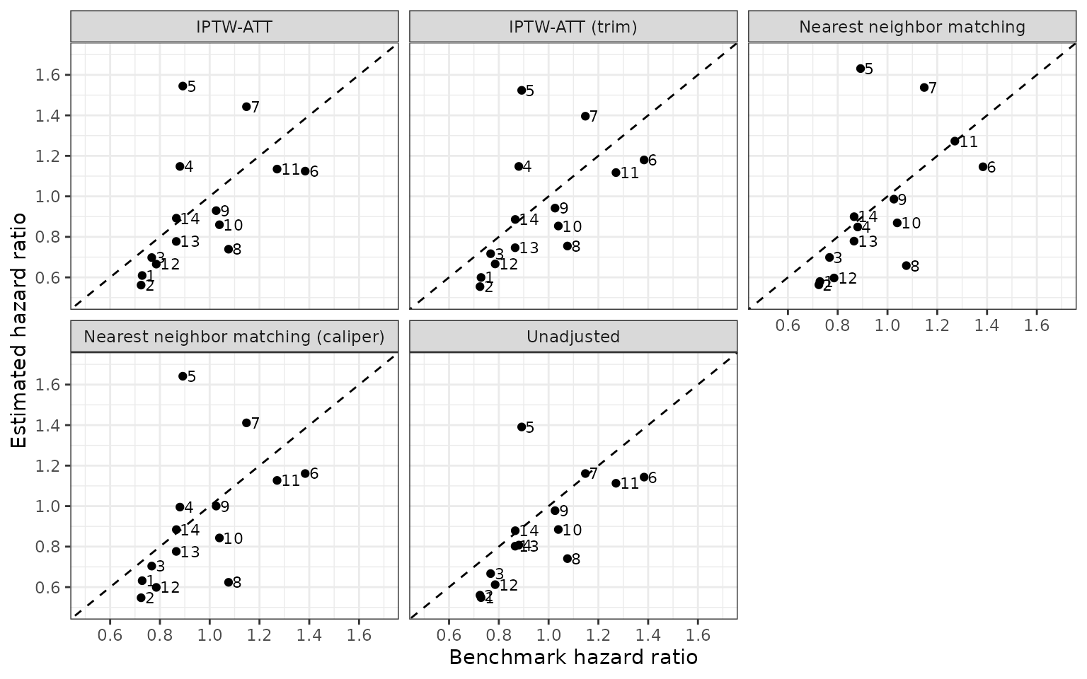
Double adjustment
Next, we use “double adjustment” to estimate log hazard ratios, which simply includes each term in the propensity score model in the Cox model as well. Note that this results in estimation of a conditional rather than a marginal hazard ratio. We leverage the update.surv_ate() function to update the analysis above while only modifying the function argument of interest.
da_ate <- update(psmethods_ate, double_adjustment = TRUE)
## Warning in coxph.fit(X, Y, istrat, offset, init, control, weights = weights, :
## Loglik converged before variable 6 ; coefficient may be infinite.

## Warning in coxph.fit(X, Y, istrat, offset, init, control, weights = weights, :
## Loglik converged before variable 6 ; coefficient may be infinite.

## Warning in coxph.fit(X, Y, istrat, offset, init, control, weights = weights, :
## Loglik converged before variable 6 ; coefficient may be infinite.

## Warning in coxph.fit(X, Y, istrat, offset, init, control, weights = weights, :
## Loglik converged before variable 6 ; coefficient may be infinite.
## Warning in coxph.fit(X, Y, istrat, offset, init, control, weights = weights, :
## Loglik converged before variable 4 ; coefficient may be infinite.

## Warning in coxph.fit(X, Y, istrat, offset, init, control, weights = weights, :
## Loglik converged before variable 4 ; coefficient may be infinite.
## Warning in coxph.fit(X, Y, istrat, offset, init, control, weights = weights, :
## Ran out of iterations and did not converge
## Warning in coxph.fit(X, Y, istrat, offset, init, control, weights = weights, :
## Loglik converged before variable 4 ; coefficient may be infinite.

## Warning in coxph.fit(X, Y, istrat, offset, init, control, weights = weights, :
## Loglik converged before variable 4 ; coefficient may be infinite.
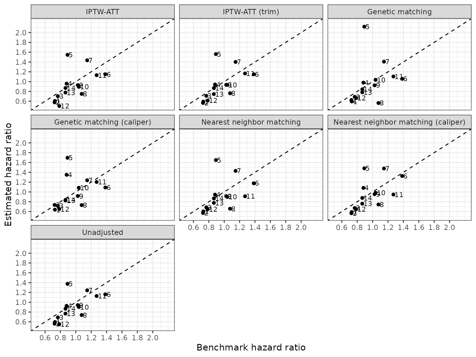
We again compare the estimated and benchmark hazard ratios.
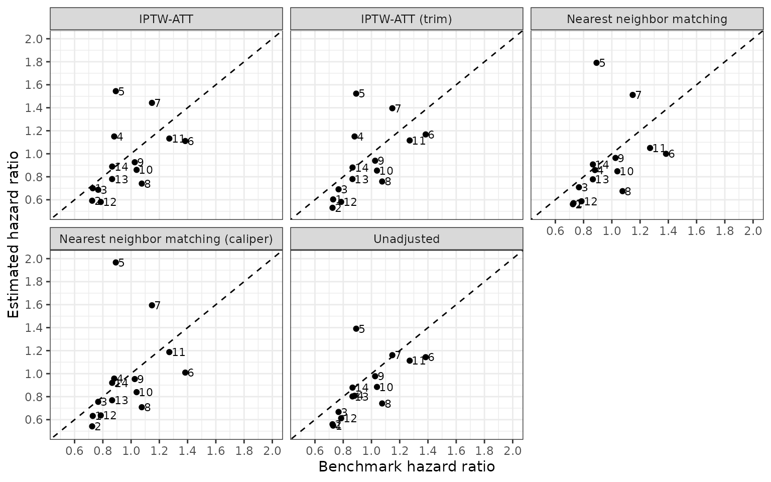
Interaction terms in the propensity score model
An additional sensitivity analysis modifies the specification of the propensity score model by interacting the number of days since diagnosis with cancer stage (early or advanced). Since we have modeled the propensity score model, we re-impute the data (including the new interaction term in the imputation model) and all propensity score modeling steps. A complete propensity score pipeline including estimation of ATEs can be performed with ps_surv() and we can iterate over groups with map_ps_surv(). Note that we don’t perform genetic matching here due to its slow run time.
These less parsimonious model results in predicted propensity scores that are either 0 or 1 as noted by the warning below, a violation of the strongly ignorable treatment assignment (SITA) assumption requiring each patient to have a nonzero probability of receiving either treatment.
ec_rct1_list <- group_split(ec_rct1, analysis_num)
ps_form_interaction <- get_ps_formula(spline = FALSE, interaction = TRUE)
interaction_ps_surv <- map_ps_surv(ec_rct1_list,
                                   formula = ps_form_interaction,
                                   ydata_list = y_list,
                                   response = RESPONSE,
                                   id = ID, grp_id = GRP_ID,
                                   integer_grp_id = TRUE)
## Warning: glm.fit: fitted probabilities numerically 0 or 1 occurred

## Warning: glm.fit: fitted probabilities numerically 0 or 1 occurred

## Warning: glm.fit: fitted probabilities numerically 0 or 1 occurred

## Warning: glm.fit: fitted probabilities numerically 0 or 1 occurred

## Warning: glm.fit: fitted probabilities numerically 0 or 1 occurred

## Warning: glm.fit: fitted probabilities numerically 0 or 1 occurred

## Warning: glm.fit: fitted probabilities numerically 0 or 1 occurred

## Warning: glm.fit: fitted probabilities numerically 0 or 1 occurred

## Warning: glm.fit: fitted probabilities numerically 0 or 1 occurred

## Warning: glm.fit: fitted probabilities numerically 0 or 1 occurred
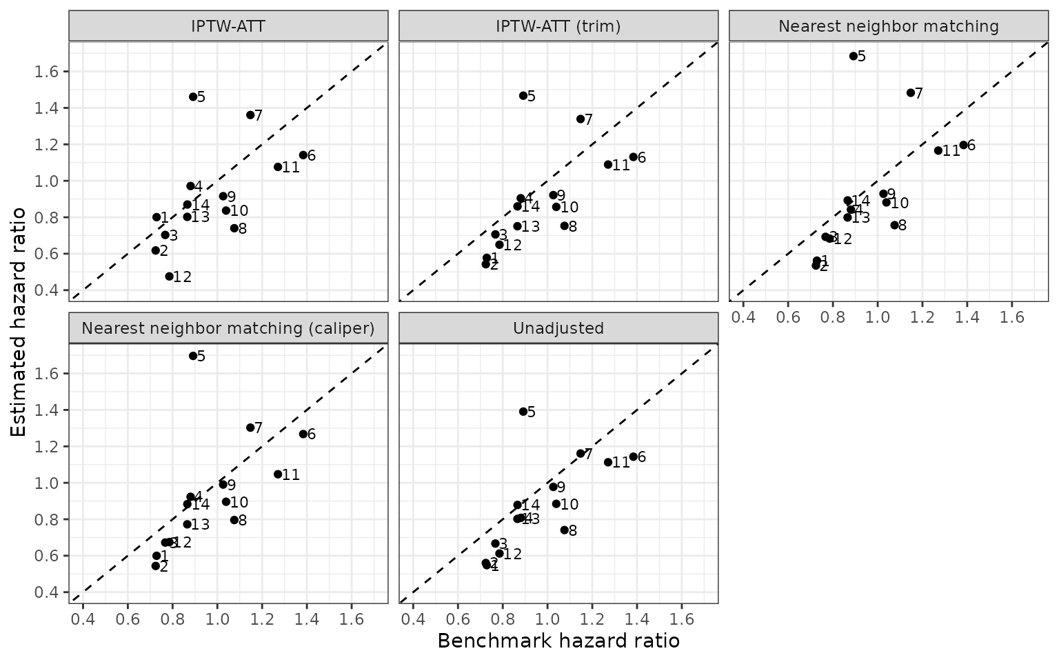
Splines in the propensity score model
We also modified the specification of the propensity score to include splines for the continuous covariates (age only), while removing the interaction term. Similar to above, we leverage the update.grouped_ps_surv() function to restimate map_ps_surv() while only modifying one argument (the propensity score model formula). This again results in some overfitting of the propensity score model.
ps_form_splines <- get_ps_formula(spline = TRUE, interaction = FALSE)
splines_ps_surv <- update(interaction_ps_surv, formula = ps_form_splines)
## Warning: glm.fit: fitted probabilities numerically 0 or 1 occurred

## Warning: glm.fit: fitted probabilities numerically 0 or 1 occurred

## Warning: glm.fit: fitted probabilities numerically 0 or 1 occurred

## Warning: glm.fit: fitted probabilities numerically 0 or 1 occurred

## Warning: glm.fit: fitted probabilities numerically 0 or 1 occurred

## Warning: glm.fit: fitted probabilities numerically 0 or 1 occurred

## Warning: glm.fit: fitted probabilities numerically 0 or 1 occurred

## Warning: glm.fit: fitted probabilities numerically 0 or 1 occurred

## Warning: glm.fit: fitted probabilities numerically 0 or 1 occurred

## Warning: glm.fit: fitted probabilities numerically 0 or 1 occurred

## Warning: glm.fit: fitted probabilities numerically 0 or 1 occurred

## Warning: glm.fit: fitted probabilities numerically 0 or 1 occurred

## Warning: glm.fit: fitted probabilities numerically 0 or 1 occurred

## Warning: glm.fit: fitted probabilities numerically 0 or 1 occurred

## Warning: glm.fit: fitted probabilities numerically 0 or 1 occurred

## Warning: glm.fit: fitted probabilities numerically 0 or 1 occurred

## Warning: glm.fit: fitted probabilities numerically 0 or 1 occurred

## Warning: glm.fit: fitted probabilities numerically 0 or 1 occurred

## Warning: glm.fit: fitted probabilities numerically 0 or 1 occurred

## Warning: glm.fit: fitted probabilities numerically 0 or 1 occurred

## Warning: glm.fit: fitted probabilities numerically 0 or 1 occurred

## Warning: glm.fit: fitted probabilities numerically 0 or 1 occurred

## Warning: glm.fit: fitted probabilities numerically 0 or 1 occurred

## Warning: glm.fit: fitted probabilities numerically 0 or 1 occurred

## Warning: glm.fit: fitted probabilities numerically 0 or 1 occurred
Splines and interaction terms in the propensity score model
In a final check of the specification of the propensity score model, we include both splines and interaction terms, which not surprisingly results in predicted propensity scores of 0 and 1.
ps_form_splines_interaction <- get_ps_formula(spline = TRUE, interaction = TRUE)
splines_interaction_ps_surv <- update(interaction_ps_surv,
                                      formula = ps_form_splines_interaction)
## Warning: glm.fit: fitted probabilities numerically 0 or 1 occurred

## Warning: glm.fit: fitted probabilities numerically 0 or 1 occurred

## Warning: glm.fit: fitted probabilities numerically 0 or 1 occurred

## Warning: glm.fit: fitted probabilities numerically 0 or 1 occurred

## Warning: glm.fit: fitted probabilities numerically 0 or 1 occurred

## Warning: glm.fit: fitted probabilities numerically 0 or 1 occurred

## Warning: glm.fit: fitted probabilities numerically 0 or 1 occurred

## Warning: glm.fit: fitted probabilities numerically 0 or 1 occurred

## Warning: glm.fit: fitted probabilities numerically 0 or 1 occurred

## Warning: glm.fit: fitted probabilities numerically 0 or 1 occurred

## Warning: glm.fit: fitted probabilities numerically 0 or 1 occurred

## Warning: glm.fit: fitted probabilities numerically 0 or 1 occurred

## Warning: glm.fit: fitted probabilities numerically 0 or 1 occurred

## Warning: glm.fit: fitted probabilities numerically 0 or 1 occurred

## Warning: glm.fit: fitted probabilities numerically 0 or 1 occurred

## Warning: glm.fit: fitted probabilities numerically 0 or 1 occurred

## Warning: glm.fit: fitted probabilities numerically 0 or 1 occurred

## Warning: glm.fit: fitted probabilities numerically 0 or 1 occurred

## Warning: glm.fit: fitted probabilities numerically 0 or 1 occurred
## Warning: glm.fit: algorithm did not converge
## Warning: glm.fit: fitted probabilities numerically 0 or 1 occurred

## Warning: glm.fit: fitted probabilities numerically 0 or 1 occurred
## Warning: glm.fit: algorithm did not converge
## Warning: glm.fit: fitted probabilities numerically 0 or 1 occurred

## Warning: glm.fit: fitted probabilities numerically 0 or 1 occurred

## Warning: glm.fit: fitted probabilities numerically 0 or 1 occurred
## Warning in predict.lm(object, newdata, se.fit, scale = 1, type = if (type == :
## prediction from a rank-deficient fit may be misleading

## Warning in predict.lm(object, newdata, se.fit, scale = 1, type = if (type == :
## prediction from a rank-deficient fit may be misleading

## Warning in predict.lm(object, newdata, se.fit, scale = 1, type = if (type == :
## prediction from a rank-deficient fit may be misleading

## Warning in predict.lm(object, newdata, se.fit, scale = 1, type = if (type == :
## prediction from a rank-deficient fit may be misleading

## Warning in predict.lm(object, newdata, se.fit, scale = 1, type = if (type == :
## prediction from a rank-deficient fit may be misleading
## Warning: glm.fit: fitted probabilities numerically 0 or 1 occurred

## Warning: glm.fit: fitted probabilities numerically 0 or 1 occurred

## Warning: glm.fit: fitted probabilities numerically 0 or 1 occurred

## Warning: glm.fit: fitted probabilities numerically 0 or 1 occurred

## Warning: glm.fit: fitted probabilities numerically 0 or 1 occurred

## Warning: glm.fit: fitted probabilities numerically 0 or 1 occurred

## Warning: glm.fit: fitted probabilities numerically 0 or 1 occurred

## Warning: glm.fit: fitted probabilities numerically 0 or 1 occurred

## Warning: glm.fit: fitted probabilities numerically 0 or 1 occurred

## Warning: glm.fit: fitted probabilities numerically 0 or 1 occurred
## Warning: glm.fit: algorithm did not converge
## Warning: glm.fit: fitted probabilities numerically 0 or 1 occurred

## Warning: glm.fit: fitted probabilities numerically 0 or 1 occurred

## Warning: glm.fit: fitted probabilities numerically 0 or 1 occurred

## Warning: glm.fit: fitted probabilities numerically 0 or 1 occurred

## Warning: glm.fit: fitted probabilities numerically 0 or 1 occurred
## Warning in predict.lm(object, newdata, se.fit, scale = 1, type = if (type == :
## prediction from a rank-deficient fit may be misleading

## Warning in predict.lm(object, newdata, se.fit, scale = 1, type = if (type == :
## prediction from a rank-deficient fit may be misleading

## Warning in predict.lm(object, newdata, se.fit, scale = 1, type = if (type == :
## prediction from a rank-deficient fit may be misleading

## Warning in predict.lm(object, newdata, se.fit, scale = 1, type = if (type == :
## prediction from a rank-deficient fit may be misleading
## Warning: glm.fit: fitted probabilities numerically 0 or 1 occurred

## Warning: glm.fit: fitted probabilities numerically 0 or 1 occurred

## Warning: glm.fit: fitted probabilities numerically 0 or 1 occurred

## Warning: glm.fit: fitted probabilities numerically 0 or 1 occurred

## Warning: glm.fit: fitted probabilities numerically 0 or 1 occurred
Missing indicators
Finally, we assessed whether combining multiple imputation with indicator variables for missing observations could reduce bias. An indicator variable was created for each variable with at least one missing observation (prior to imputation) and given a value of 1 if it was missing and 0 otherwise.
missing_indicator_ps_surv <- update(interaction_ps_surv,
                                    formula = analysis$ps_formula,
                                    missing_dummy = TRUE)
Summary of primary and sensitivity analyses
Finally, we combine the hazard ratios across both the primary and the sensitivity analyses. We summarize the estimates across 14 pairwise comparisons by computing the root mean square error (RMSE) in comparisons of the estimated hazard ratios and RCT benchmarks. The “unadjusted” estimates surprisingly perform the best.
sensitivity_lookup <- tribble(
   ~id, ~Type,  ~`PS specification`, ~`Double adjustment`, ~`Missing data`,
   "1", "Primary", "No interaction or splines", "No", "Multiple imputation",
   "2", "Sensitivty", "No interaction or splines", "No", "Multiple imputation",
   "3", "Sensitivty", "No interaction or splines", "Yes", "Multiple imputation",
   "4", "Sensitivty", "No interaction or splines", "Yes", "Multiple imputation",
   "5", "Sensitivty", "Splines and no interaction", "No", "Multiple imputation",
   "6", "Sensitivty", "Splines and interaction", "No", "Multiple imputation",
   "7", "Sensitivty", "No interaction or splines", "No", "Multiple imputation + missing indicator"
)

hr <- list(
  `1` = primary_hr,
  `2` = psmethods_hr %>%
    filter(method != "iptw_att_trim"),
  `3` = da_hr,
  `4` = interaction_hr,
  `5` = splines_hr,
  `6` = splines_interaction_hr,
  `7` = missing_indicator_hr
) %>%
  bind_rows(.id = "id") %>%
  left_join(sensitivity_lookup, by = "id")

rmse <- function(estimate, truth) {
  sqrt(mean((estimate - truth)^2))
}

hr %>%
  group_by(Type, method, `PS specification`, `Double adjustment`,
           `Missing data`) %>%
  summarise(rmse = rmse(estimate, benchmark_estimate)) %>%
  mutate(method = label_ps_method(method)) %>%
  arrange(rmse) %>%
  rename(`PS method` = method, RMSE = rmse) %>%
  html_table()
|
Type
|
PS method
|
PS specification
|
Double adjustment
|
Missing data
|
RMSE
|
|
Sensitivty
|
Unadjusted
|
No interaction or splines
|
Yes
|
Multiple imputation
|
0.2023242
|
|
Sensitivty
|
Unadjusted
|
No interaction or splines
|
No
|
Multiple imputation
|
0.2034054
|
|
Sensitivty
|
Unadjusted
|
No interaction or splines
|
No
|
Multiple imputation + missing indicator
|
0.2034054
|
|
Sensitivty
|
Unadjusted
|
Splines and interaction
|
No
|
Multiple imputation
|
0.2034054
|
|
Sensitivty
|
Unadjusted
|
Splines and no interaction
|
No
|
Multiple imputation
|
0.2034054
|
|
Sensitivty
|
IPTW-ATT (trim)
|
No interaction or splines
|
No
|
Multiple imputation + missing indicator
|
0.2243540
|
|
Primary
|
IPTW-ATT (trim)
|
No interaction or splines
|
No
|
Multiple imputation
|
0.2247665
|
|
Sensitivty
|
Nearest neighbor matching (caliper)
|
No interaction or splines
|
No
|
Multiple imputation
|
0.2301874
|
|
Sensitivty
|
IPTW-ATT
|
No interaction or splines
|
No
|
Multiple imputation + missing indicator
|
0.2331015
|
|
Sensitivty
|
IPTW-ATT
|
No interaction or splines
|
No
|
Multiple imputation
|
0.2331830
|
|
Sensitivty
|
IPTW-ATT (trim)
|
No interaction or splines
|
Yes
|
Multiple imputation
|
0.2336454
|
|
Sensitivty
|
Genetic matching (caliper)
|
No interaction or splines
|
No
|
Multiple imputation
|
0.2338702
|
|
Sensitivty
|
IPTW-ATT
|
No interaction or splines
|
Yes
|
Multiple imputation
|
0.2379320
|
|
Sensitivty
|
IPTW-ATT (trim)
|
Splines and no interaction
|
No
|
Multiple imputation
|
0.2418070
|
|
Sensitivty
|
Nearest neighbor matching (caliper)
|
No interaction or splines
|
Yes
|
Multiple imputation
|
0.2439931
|
|
Sensitivty
|
IPTW-ATT (trim)
|
Splines and interaction
|
No
|
Multiple imputation
|
0.2469538
|
|
Sensitivty
|
IPTW-ATT
|
Splines and no interaction
|
No
|
Multiple imputation
|
0.2526150
|
|
Sensitivty
|
IPTW-ATT
|
Splines and interaction
|
No
|
Multiple imputation
|
0.2546834
|
|
Sensitivty
|
Nearest neighbor matching (caliper)
|
No interaction or splines
|
No
|
Multiple imputation + missing indicator
|
0.2558140
|
|
Sensitivty
|
Nearest neighbor matching
|
No interaction or splines
|
Yes
|
Multiple imputation
|
0.2674952
|
|
Sensitivty
|
Nearest neighbor matching
|
No interaction or splines
|
No
|
Multiple imputation + missing indicator
|
0.2683666
|
|
Sensitivty
|
Nearest neighbor matching (caliper)
|
Splines and no interaction
|
No
|
Multiple imputation
|
0.2733221
|
|
Sensitivty
|
Nearest neighbor matching
|
Splines and no interaction
|
No
|
Multiple imputation
|
0.2748839
|
|
Sensitivty
|
Genetic matching (caliper)
|
No interaction or splines
|
Yes
|
Multiple imputation
|
0.2840310
|
|
Sensitivty
|
Nearest neighbor matching
|
No interaction or splines
|
No
|
Multiple imputation
|
0.2840818
|
|
Sensitivty
|
Nearest neighbor matching
|
Splines and interaction
|
No
|
Multiple imputation
|
0.3209607
|
|
Sensitivty
|
Genetic matching
|
No interaction or splines
|
No
|
Multiple imputation
|
0.3398841
|
|
Sensitivty
|
Nearest neighbor matching (caliper)
|
Splines and interaction
|
No
|
Multiple imputation
|
0.3551631
|
|
Sensitivty
|
Genetic matching
|
No interaction or splines
|
Yes
|
Multiple imputation
|
0.3824202
|